4. Excel How to remove duplicates ?
Excel makes it easy to remove duplicates using the Remove Duplicates button in the Data Tools group on the Data tab of the Ribbon.
Example
For example, let's take the following list:
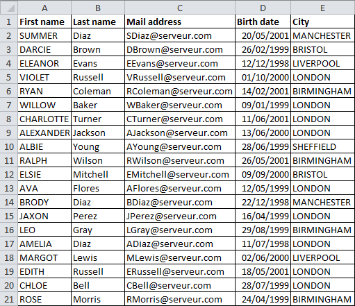
How to remove duplicates
Select any cell in the list.
Click the Remove Duplicates button in the Data Tools group on the Data tab of the Ribbon.

This opens the Remove Duplicates dialog box. In this dialogue box, I define how lines are considered duplicate:
- If I consider lines with the same e-mail address to be duplicates, then I only check the "E-mail address" box
- If I consider that rows with the same last name, first name and date of birth are duplicates, then I have to check the checkboxes for these three columns.

Validate with the OK button.
With this method, for each duplicate, Excel
- leaves the first occurrence intact, i.e. the first line of each duplicate
- deletes the other occurrences.
However, if you only want Excel to highlight the duplicates without deleting them, then you should use conditional formatting.
Highlighting duplicate lines using conditional formatting
Duplicate values in the "Mail Address" column
Normally, there should not be any duplicate e-mail addresses, otherwise it is a data entry error. So let's use the conditional formatting technique to find and correct any duplicates.
Select column C and click on the Conditional Formatting command on the Home tab of the Ribbon, choose Highlight Cells Rules, then choose Duplicate Values.

Excel highlights duplicate values in the selection.
Duplicate values in relation to the last name, first name and date of birth columns
I now consider rows to be duplicates when they have the same last name, first name and date of birth.
This problem cannot be solved by selecting all 3 columns and using the Duplicate Values command in Conditional Formatting. However, a very simple trick is to record a concatenation of the values of the 3 columns in another column.
For example, enter the following formula in cell F2 and copy it to column F by Auto Filling:
=A2 & "__" & B2 & "___" & D2
Then apply the Duplicate Values command in Conditional Formatting to column F.

A small problem with this method is that the values are highlighted in column F and not in the original table. A solution to this problem is given in the form of an exercise: Finding duplicates
See also the chapter Conditional Formatting.