20. Excel How to compare two columns ? How do I fill in one sheet from another ?

---

Comparison of two columns

Consider the following spreadsheet with a list of employees:

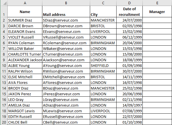
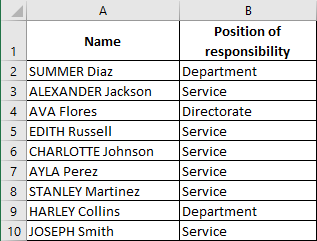
We want to fill in column E "Manager" with the word "Yes" for the managers of the organisation. The list of managers is written in another sheet "Sheet2":

I assume that the two sheets belong to the same workbook, and that column A "Name" does not contain any duplicates.

The formula to be written in cell E2 and copied to column E by Autofill :

=IF(COUNTIF(Sheet2!$A$2:$A$179,A2)>0,"Yes","")

Completing one sheet from another

Using the VLOOKUP function

In the previous example, we added "Yes" for the organisation's managers. We now want to add the responsibility position for each manager by extracting it from column B of the sheet "Sheet2".

To do this we will use the formula :

=VLOOKUP(A2,Sheet2!$A$1:$B$179,2,FALSE)

But as we can see from the following extract, the result is not satisfactory:

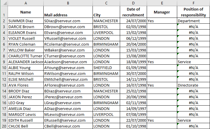
Indeed, the function VLOOKUP returns the error #N/A when the searched value is not found.

The solution is to use the IFERROR function. This function returns the value of its 1^st argument if it is not an error. Otherwise, the function returns the value of its 2^nd argument. So, in this case, I give the empty string "" as the 2^nd argument.

The formula in F2 to be copied to column F by Autofill is :

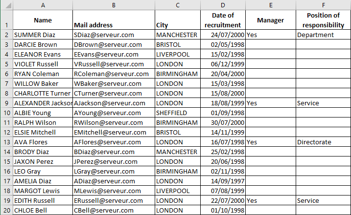
=IFERROR(VLOOKUP(A2,Sheet2!$A$1:$B$179,2,FALSE),"")

The result:

Using the MATCH and INDEX functions

The same problem can be solved using the formula :

=INDEX(Sheet2!$A$2:$B$179,MATCH(A2,Sheet2!$A$2:$A$179,0),2)

The MATCH function in this formula returns the position of the value in A2 in the range A2:A179 of the sheet "Sheet2".

INDEX returns the value in the range A2:B179 of the sheet "Sheet2" in the intersection of

• the row whose number is the value returned by MATCH and
• column 2.

But, once again, the MATCH function returns the error #N/A when the searched value is not found.

In order not to have this error displayed, use preferably the formula :

=IFERROR(INDEX(Sheet2!$A$2:$B$179,MATCH(A2,Sheet2!$A$2:$A$179,0),2),"")

---