2. Exercise 2 – Formatting

---

Prerequisites

It is advisable to read the Excel 2016 Course up to the 4^th chapter Formatting before starting this exercise.

Question

Reproduce the following spreadsheet excerpt with formatting:

You can download the file for this exercise here.

---

Indications Exercice 2 – Formatting

---

1 - Merge the following ranges

• A1:F1
• A4:F4
• A12:F12
• A17:F17
• A21:E21
• A22:E22
• A23:E23

I remind you that you can of course merge each range one after the other. But, you can also, select all these ranges simultaneously and use the Merge Across button which will merge cells in each row apart:

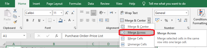
2 - Select the merged cell in A1:F1 and

• Set the font size to 18
• Bold and underlined text
• Center the text horizontally
• White font color
• Dark gray fill color

3 - Select the range A3:F3 and

• Text in bold italics
• Center the text horizontally
• White font color
• Fill color Dark blue
• White interior border

4 - Simultaneously select the ranges A4:F4, A12:F12 and A17:F17 and

• Bold text
• Fill color Light blue

5 - Simultaneously select the ranges A21:E21, A22:E22 and A23:E23 and

• Bold text
• Align text horizontally to the right
• Fill color Light gray

6 - Select range A4:F23 and apply thick outside and inside border

7 - Simultaneously select the ranges E5:F11, E13:F16, E18:F20 and F21:F23 and define the number format Comma Style

8 - Select columns A to F. Double-click on the edge of one of the headers of columns A to F to automatically adjust the column widths.

---