9. Data manipulation

In this chapter, we will see techniques for working with data, including

Data sorting
Data filtering
Validating data
Adding subtotals

Consider the following workbook extract:

You can download this file here

9.1. Sorting data

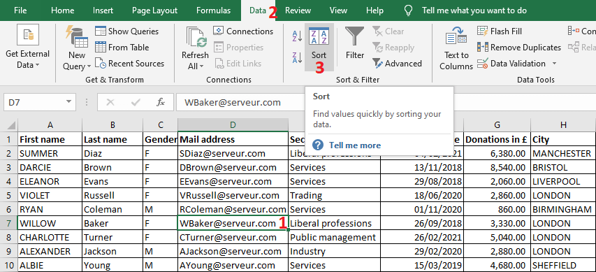
For example, let's sort this list by membership date. To do this:

Select a cell in the "Membership date" column
Click on the Data tab of the ribbon
Click on the Sort Oldest to Newest command. Or click on the Sort Newest to Oldest button; depending on which way you want to sort the list

NOTE. The Sort commands are also available on the Home tab of the ribbon; following the path: Home tab/Sort & filter/Sort...

For example, we want to sort according to the date of membership but with each sector separately. We must therefore sort according to the sector and according to the date of membership as follows:

Select any cell in the list
Click on the Data tab of the ribbon
Click on the Sort command

The Sort dialog box appears. Make sure that the box My data has headers is checked.
Select the "Sector" column in the Sort by list.
Then click on the Add Level button.

A second level of sorting is added. Select the column "Membership date" in the list Then by.
Finally validate by clicking on the OK button.

NB. You can, of course, add other sorting levels.

9.2. Data filtering

This technique allows us to display a subset of our data list according to one or more criteria. For example, we want to display only :

Female members
Members from one or more sectors
People who joined in 2016 for example
As we can also make a combination of two or more criteria

Here is how to do it:

Select a cell in your list
Click on the Data tab of the ribbon
Click on the Filter command
The column headers will have buttons that allow you to open a filter menu , cliquez par exemple sur le bouton à l’entête de la colonne « Secteur d’activité »

A list of unique values sorted in order is displayed, with a checkbox in front of each value.
Click the Select All checkbox to uncheck all checkboxes
Click on the checkbox or checkboxes you want. For example, check the boxes for "Trading" and "Services".
Validate with the OK button. Note that only the rows with one or the other of the values "Trading" and "Services" are displayed in the "Sector" column.

You can add other criteria. For example, to display the members of the "Trading" and "Services" activity sectors living in "London":

Click on the button opening the filtering menu at the top of the "City" column
Click on the Select All checkbox to uncheck all checkboxes
Click on the "London" checkbox

Click on the OK button to validate. Notice that at the bottom of the screen, Excel displays the number of records (= rows) found:

Now I invite you to see the options in the Text Filters menu. Click on the button to open the filter menu at the header of a column filled with plain text (without dates or numbers), for example the "Activity sector" column, then on the Text Filters menu :

Also note the options available for a column of type Numbers. Click on the button to open the filter menu at the header of the "Donations in £" column, then on the Number Filters menu:

Also note the options available for a column of type Dates. Click on the button to open the filter menu in the column header "Membership date", then on the menu Date Filters :

To cancel the filtering of a column:

Click on the button opening the filtering menu at the header of a column involved in the filtering. For example, the Sector column
Click on the Clear filter from "Sector" command

NOTE. To cancel all filters, click on the Filter button on the Data tab.

9.3. Data validation

Data validation is a possibility that allows us to impose restrictions on the values accepted in a column. We can, for example, impose that the values entered in a column are numbers in a desired range of values. This is also useful when a column can only take a limited number of values, as is the case with the "Gender" column, which must only have the values M or F.

But why impose constraints, especially if I am the one who is going to fill my file?

Normally, whether it is you who fills in the file or you give it to other people to fill in, you should know that mistakes happen everywhere and that we need to work rapidly. For a date column, for example, you mistakenly enter values like "30/02/2018" or "11/15/2018". In this case, Excel will tell you right away that the value entered is not correct.

As we will see with examples, there is a possibility to display an explanatory message, as soon as the cell in question is active. We can also specify an error message that is displayed when an incorrect value is entered.

Let's consider the same example from this chapter:

Select the "Membership Date" column
Click on the Data tab of the ribbon
Click on the Data Validation command. The Data Validation dialog box will open

In the Data Validation dialog box:

Choose "Date" from the Allow list.
NOTE. Fields are added according to the value chosen from the Allow list.
For the Data list, let's leave the option "between".
Assuming that the association designated by this workbook was created on 05/01/2018, no one has joined before this date. Therefore, in the Start date field of the Data validation dialog box, let's set the value "05/01/2018".
In the End date field, let's set the value to "=TODAY()". The predefined function TODAY returns today's date; the one configured in your Windows system.
Finally, go to the Input Message tab of this dialog box

The Input Message tab of the Data Validation dialog box allows you to define a message that appears when the cell in question is selected:

Enter a Title
Enter an Input message
Then go to the Error Alert tab of this dialog box

The Error Alert tab of the Data Validation dialog box allows you to define a message that appears when a value that does not respect the validation rule is entered in a cell concerned by this validation:

Enter a Title
Enter an Error message
Then validate by clicking on the OK button.

It is also possible to validate data against a list of values. This is appropriate for the columns "Gender", "Sector" and "City" in our example, each of which accepts a limited number of values.

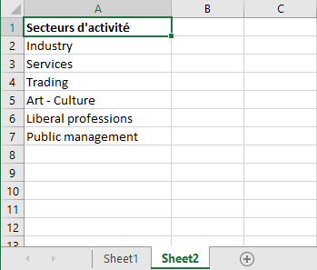
Let's illustrate this with the case of the "Sector" column. Let's start by entering the values in a range of cells. And since I prefer to enter this list in another sheet, I will first :

Add a new worksheet. To do this, click on the Add Sheet button at the bottom left of the Excel window
To the created sheet, enter the values as follows:

Reactivate sheet 1; click on the tab of sheet1 at the bottom left of the Excel window
Select the "Sector" column
Open the Data Validation dialog box
Choose "List" from the Allow list. Leave the "Ignore blank" and "In-cell dropdown" boxes checked
In the Source field of the dialog box, enter the address of the range A2:A7 on sheet 2, where we entered the list of sector values. I remind you that if you want Excel to add this address :
- Click at the Source field in the Data Validation dialog box.
- Reactivate Sheet2; click on the Sheet2 tab at the bottom left of the Excel window
- Select the cell range A2:A7
- Validate by clicking on the OK button.

Here you can also add an input message and an error alert as in the previous example.

Now check the effect of your configuration:

Click on a cell in the "Sector" column. Notice the button that appears to the right of the cell
Click on this button to open the list. Notice that the list contains the entries you entered in range A2:A7 on Sheet 2
Click on an entry in the list and notice that this value is written to the cell

9.4. Adding subtotals

Let's use the same example and add subtotals for "Donations" by "City" and "Sector".

However, in this case, we need to sort by "City" and "Sector". I remind you of the procedure for doing this sorting:

Click on a cell in the data list
Click on the Data tab
Click on the Sort command. The Sort dialog box appears.

In the Sort dialog box :

Make sure that the box My data has headers is checked.
Select the "City" column in the Sort by list.
Then click on the Add Level button.

A second level of sorting is added. Select the column "Sector" in the list Then by.
Finally, validate by clicking on the OK button.

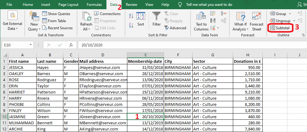
Now let's add the subtotals for "Donations" by "City" and by "Sector":

Click on a cell in the data list
Click on the Data tab
Click on the Subtotal command. The Subtotal dialog box appears.

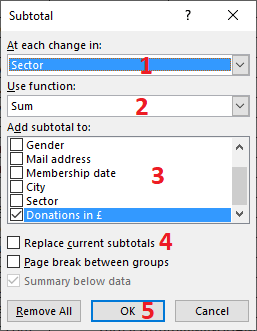
In the Subtotal dialog box that appears:

Select "City" from the list At each change in
Select "Sum" from the Use function list
Check "Donations in £" from the list Add subtotal to
Click on the OK button

Notice the addition to your sheet of a row with a subtotal for each value change in the "City" column. Also notice the addition of grouping symbols on the left side of the Excel window. Click on each of these grouping symbols , , , and to see the result.

Now let's add the subtotals by "Sector". To do this, click once again on the Subtotal button on the Data tab of the Ribbon. The Subtotal dialog box will appear. Fill it in as follows:

Select "Sector" from the list At each change in
Select "Sum" from the Use Function list
Check "Donations in £" from the Add subtotal to list
Uncheck Replace current subtotals, so that Excel does not override the previous subtotal
Click on the OK button

Notice the addition of subtotals by "City" and by "Sector". And notice the addition of the fourth level for grouping symbols.

<< 8. Work with spreadsheets

10. Generation of graphics >>

Reader comments