7. Exercise - Finding duplicates
Prerequisites
It is advisable to read the Excel 2016 Course up to the 7th chapter Conditional formatting before starting this exercise.
Question
Consider the following spreadsheet extract:
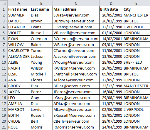
Using the Conditional Formatting technique, I propose to highlight the duplicate rows in this table by considering that rows are duplicated when they have the same last name, first name and date of birth.
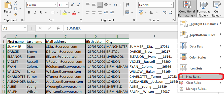
This problem cannot be solved by selecting the 3 columns and using the Duplicate Values command in Conditional Formatting. However, a very simple trick is to record a concatenation of the values of the 3 columns in another column.
For example, enter the following formula in cell F2 and copy it to column F by Auto Filling:
=A2 & "__" & B2 & "___" & D2
If you apply the Duplicate Values command in Conditional Formatting to column F, then the duplicate values in column F will be highlighted. But, how do you highlight the duplicate rows in the original table (Columns A-E) and not in column F?
Indications Exercise – Finding duplicates
Select the cell range A2:E1475. Click the Conditional Formatting command on the Home tab of the Ribbon and choose New Rule...
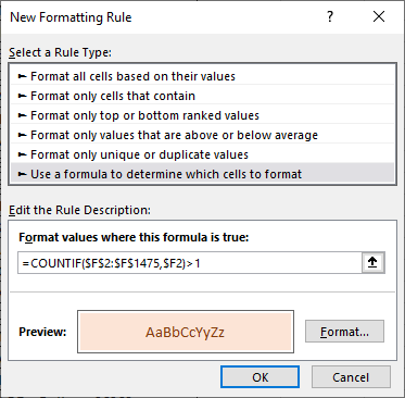
In the New Formatting Rule dialog box that appears :
- Click on Use a formula to determine which cells to format from the list Select a Rule Type...
- In the Format values where this formula is true field enter the formula :
=COUNTIF($F$2:$F$1475,$F2)>1
- Then click on the Format... button to open the Format Cells dialog box and choose the format that suits you.
- Confirm with the OK button.
Explanations about the formula:
The function COUNTIF will count the number of occurrences of the value in cell F2 in the range F2:F1475 i.e. the filled range of column F. Of course, it will count the value in F2. So when there is more than one occurrence, then the value is duplicated.
I remind you that the formula must be written in relation to the 1st cell of the selection. That is to say, the one located at the top left of the selection; i.e. A2. And considering that this formula will be applied by Excel to the rest of the selection in a similar way to that of the Auto Filling.
So, as far as the 2nd argument $F2:
- I put the "$" in front of the "F" because otherwise in cell B2, Excel will count the occurrences of the value in cell G2 and not the one in cell F2
- I did not put the "$" in front of the "2" because otherwise in all rows, Excel will count the occurrences of the value in cell F2.