12. Excel How to have alternating row colours?

---

We can have alternating colours of the rows of an Excel sheet in one of three ways:

• Use the Format Painter button,
• Create an Excel table, or
• Use Conditional Formatting

Using the Format Painter button

1. Select the cells in the first row and set the colour you want.
2. Select the cells in the second row and set the colour you want.
3. Then select these first two rows and click the Format Painter button in the Clipboard group on the Home tab of the Ribbon.
4. Now click on the third row and without releasing the mouse button, move the pointer to the last line of your sheet and release the mouse button.

The disadvantage of this method compared to the following two methods is that if you delete a row from the sheet, then you have to redo steps 3 and 4.

Creating an Excel table

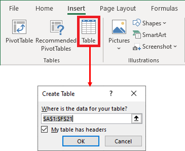
1. Select a cell in the range where you want to have the alternating colours.
2. Click the Table button in the Tables group on the Insert tab of the Ribbon.
3. The Create Table dialog box is opened. In this box, you can select another range of cells or accept the one proposed by Excel in the field Where is the data in your table?
4. Confirm with the OK button.

You will then have a formatting with alternating colours for the selected range of cells and buttons on the column headers for filtering and sorting.

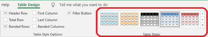
To choose another colour for your table

Click on a cell in the table. The Table Design tab is added to the Ribbon. In the Table Styles group, click on the style you want.

Using conditional formatting to have alternating colours

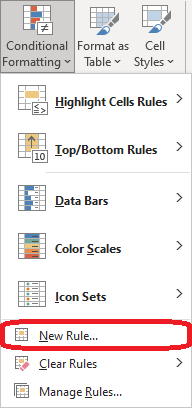
Select the range where you want to have alternating colours. Click the Conditional Formatting command on the Home tab of the Ribbon and choose New Rule....

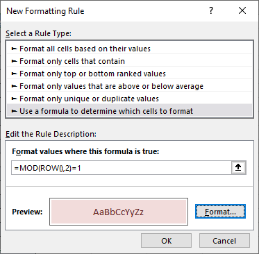
In the New Formatting Rule dialog box that appears :

• Click on Use a formula to determine which cells to format from the list Select a Rule Type...
• In the Format values where this formula is true field enter the formula :

=MOD(ROW(),2)=1

According to this formula, the format will be applied to the odd-numbered rows.

• Then click on the Format... button to open the Format Cells dialog box and choose the format you want.
• Confirm with the OK button.

Explanation of the formula

The function ROW() returns the number of the current row. The first row at the top of the sheet is numbered 1 and so on.

The function MOD returns the remainder of the integer division of the first argument by the second argument. Since this second argument is 2, then the function will return 0 when the first argument is even and return 1 when the first argument is odd.

The comparison with 1 gives a Boolean value:

• False when the current row has an even number
• True when the current row has an odd number

---

---