1. Exercise 1 – Formatting
Prerequisites
It is advisable to read the Excel 2016 Course up to the 4th chapter Formatting before starting this exercise.
Question 1
Reproduce the following worksheet excerpt:

Question 2
Change the formatting as follows:

Indications Exercise 1 – Formatting
Question 1
To reproduce the extract mentioned, you must:
1 - Merge the ranges of cells:
- A1:A2
- B1:B2
- C1:C2
- D1:G1
I remind you that to merge a range of cells, you must select it, then click on the Merge & Center command in the Alignment group on the Home tab of the ribbon.

2 - Make the text of the cell ranges bold:
- A1:G2
- A1:A10
- A10:G10
To do this, select these 3 ranges of cells simultaneously. I remind you how:
- Select the range A1:G2
- Hold down the Ctrl key on the keyboard
- Select the range A2:A9, then the range A10:G10
- Release the Ctrl key on the keyboard
Then click on the Bold command of the Font group of the Home tab of the ribbon

3 - Widen columns A, B and C.
Question 2
1 - Simultaneously select the ranges A1:G2 and A10:G10 and:
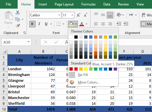
- Add the fill color in blue. To do this, click on the small arrow of the Fill Color button in the Font group of the Home tab of the ribbon. Choose the blue color from the menu that appears:

- Then apply the color white to the text. To do this, click on the small arrow of the Font color button in the Font group of the Home tab of the ribbon. Choose the White color from the menu that appears

- Increase the font size to 14. Using the keyboard, enter the value 14 in the Font size field in the Font group of the Home tab of the ribbon. Confirm with the Enter key on the keyboard. An alternative is to click on the Increase Font Size button several times until you have the desired size

- Apply borders. To do this, click on the small arrow of the Borders button in the Font group of the Home tab of the ribbon. Click on More Borders… on the menu that appears:

The Format Cells dialog box is open to the Border tab:
- Select White color
- Click on the Inside button
- Click on the OK button

2 - Select cell B1 and click the Wrap Text button in the Alignment group on the Home tab of the ribbon

3 - Select the range A3:G9 and apply the borders by clicking on the All Borders button:

4 -Simultaneously select the ranges A4:G4, A6:G6 and A8:G8. Apply a Blue-Gray fill color:

5 - Select the range C3:C10 and click on the Percent Style button in the Number group of the Home tab of the ribbon

The values in this range are now displayed as a percentage but without a decimal point. To add a digit after the decimal point, click on the Increase Decimal button:
