9. Exercise - Text Functions
Prerequisites
You should read the Excel Functions course up to the chapter Text Functions before starting this exercise.
Question
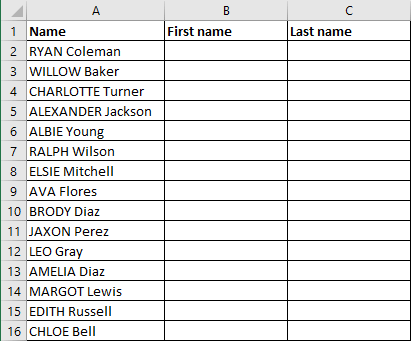
Consider the following worksheet extract where "first names last names" is written in column A.
The first names and last names are written separated by a space character. Compound names are joined by a dash and not separated by a space.
Write the appropriate formulas to have in column B the "first names" and in column C the "last names".

NB. This problem can be solved with the help of the Excel Convert Text to Columns Wizard. You can call this wizard using the Text to Columns command on the Data tab of the Ribbon. However, I ask you to solve it using formulas; this is a very good example of using Excel's text functions.
Indications Exercise - Text Functions
1 - Formula in cell B2 to extract first names?
Solution :
=MID(A2, 1, FIND(" ", A2)-1)
Explanations :
The first name is part of the text in cell A2, so I use the Excel function MID to extract a part of a string.
I give this string as the first argument, so the address of cell A2.
In the 2nd argument, it is 1, since the first name is written at the beginning of the value in cell A2; starting from the 1st character. So :
=MID(A2, 1, ----------)
In the third argument, it is the number of characters of the first name. In line 2, it is 5. But, let's not forget that we are going to make an Autofill to fill the cells of column B and the number of characters of the first name varies from one line to another.
The solution is to refer to the position of the space character in the string in cell A2. This is the Excel function FIND which returns the position of a character in a text. So the formula for finding the position of the space character is:
FIND(" ", A2)
For the number of characters in the first name, I must subtract 1 to avoid counting the space character:
FIND(" ", A2)-1
The overall formula in B2 is :
=MID(A2, 1, FIND(" ", A2)-1)
NB. Here we have an example of a nested call of functions; indeed, the result of the function FIND is given as an argument for the call of the function MID. We can avoid this nested call in the following way:
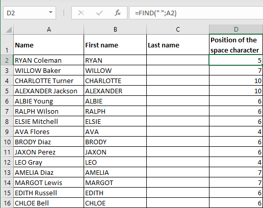
In cell D2 for example, write the formula :
=FIND(" ", A2)
If you want to show the object in column D, enter as column header in cell D1: Position of the space character.
You can then write in B2 the formula :
=MID(A2, 1, D2-1)

2 - Formula in cell C2 to extract last names?
Solution :
=MID(A2, FIND(" ", A2) + 1, LEN(A2) - FIND(" ", A2))
Explanations :
We still use the MID function to extract a part of a string.
The 2nd argument is :
FIND(" ", A2) + 1
This is the position after (hence the +1) the space character, since the last name is written in cell A2 after the space character.
As for the 3rd argument, it must be the number of characters in the last name. But, I remind you that for the MID function, when you need to extract the characters at the end of the string, it is possible to give a larger number in the 3rd argument and Excel will return the remaining characters, i.e. up to the end of the string in A2. I give for example 100, since no name has more than 100 characters.
We can therefore write in C2 the formula :
=MID(A2, FIND(" ", A2) + 1, 100)
On the other hand, it is possible to calculate exactly the number of characters in the name. To do this, you must use the LEN function, which returns the number of characters in a string. The number of characters in the last name is :
LEN(A2) - FIND(" ", A2)
I have subtracted the number of characters up to the space character from the number of characters in the text in A2.
hence the formula in C2 :
=MID(A2, FIND(" ", A2) + 1, LEN(A2) - FIND(" ", A2))
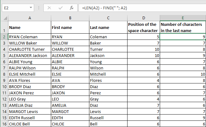
NB. To avoid having nested function calls, you can also use formulas in intermediate cells. In the case of the extract below, the formula in D2 is :
=FIND(" ", A2)
The formula in E2 is :
=LEN(A2) - FIND(" ", A2)
The formula in C2 is :
=MID(A2, D2 + 1, E2)
